3.4.2 - Edge Detection (Sobel Operator)

Duration:

20-25 minutes

Level:

Beginner

Prerequisites:

Module 1.1 (Pixel Basics), Module 3.4.1 (Convolution)

Overview

Edge detection is one of the most fundamental operations in image processing and computer vision. Edges represent boundaries between different regions in an image, where pixel intensity changes rapidly. In this exercise, you will learn how to detect edges using the Sobel operator, a classic gradient-based approach that remains widely used today.

Learning Objectives

By completing this module, you will:

• Understand what edges are and why detecting them is useful

• Learn how the Sobel operator uses gradient kernels to find edges

• Apply convolution with 3x3 kernels to compute directional gradients

• Create edge-detected images using pure NumPy operations

Quick Start: See Edge Detection in Action

Let’s begin by seeing edge detection work on a simple test image. Run the following code to detect edges in shapes we create procedurally:

Simple edge detection with Sobel operator

import numpy as np
from PIL import Image

# Create a test image with geometric shapes (256x256 grayscale)
height, width = 256, 256
image = np.zeros((height, width), dtype=np.float64)

# Draw a white rectangle and circle
image[80:180, 60:120] = 255
center_y, center_x, radius = 128, 180, 40
y_coords, x_coords = np.ogrid[:height, :width]
circle_mask = (x_coords - center_x)**2 + (y_coords - center_y)**2 <= radius**2
image[circle_mask] = 255

# Define Sobel kernels
sobel_gx = np.array([[-1, 0, 1], [-2, 0, 2], [-1, 0, 1]])
sobel_gy = np.array([[-1, -2, -1], [0, 0, 0], [1, 2, 1]])

# Apply edge detection
edge_magnitude = np.zeros((height, width), dtype=np.float64)
for y in range(1, height - 1):
    for x in range(1, width - 1):
        neighborhood = image[y-1:y+2, x-1:x+2]
        gx = np.sum(sobel_gx * neighborhood)
        gy = np.sum(sobel_gy * neighborhood)
        edge_magnitude[y, x] = np.sqrt(gx**2 + gy**2)

# Normalize and save
edge_normalized = (255 * edge_magnitude / edge_magnitude.max()).astype(np.uint8)
Image.fromarray(edge_normalized, mode='L').save('edge_detection_output.png')

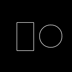
The Sobel operator detects edges as bright lines where intensity changes rapidly. Notice how both the rectangle and circle boundaries are clearly visible as white outlines.

Tip

Notice how the edges appear as white lines on a black background. The brighter the line, the stronger the edge. Areas with uniform intensity (inside the shapes or in the background) remain black because there is no change to detect.

Core Concepts

Concept 1: What is Edge Detection?

An edge in an image is a location where pixel intensity changes sharply. Think of edges as the boundaries between different regions: where a white shape meets a black background, where one color transitions to another, or where a shadow begins.

Edge detection is fundamental because:

• Object recognition: Edges define object shapes and boundaries

• Feature extraction: Computer vision algorithms use edges as landmarks

• Image segmentation: Edges help separate objects from backgrounds

• Artistic effects: Edge detection creates striking outline drawings

Mathematically, we detect edges by computing the gradient of the image, which measures how rapidly pixel values change from one location to another [GonzalezWoods2018].

Concept 2: The Sobel Operator

The Sobel operator detects edges by computing gradients in two directions using convolution kernels. Named after Irwin Sobel, who developed it in 1968, it remains one of the most widely used edge detection methods [Sobel1968].

The Sobel operator uses two 3x3 kernels:

Gx (Horizontal Gradient) - Detects vertical edges:

[-1  0  1]
[-2  0  2]
[-1  0  1]

Gy (Vertical Gradient) - Detects horizontal edges:

[-1 -2 -1]
[ 0  0  0]
[ 1  2  1]

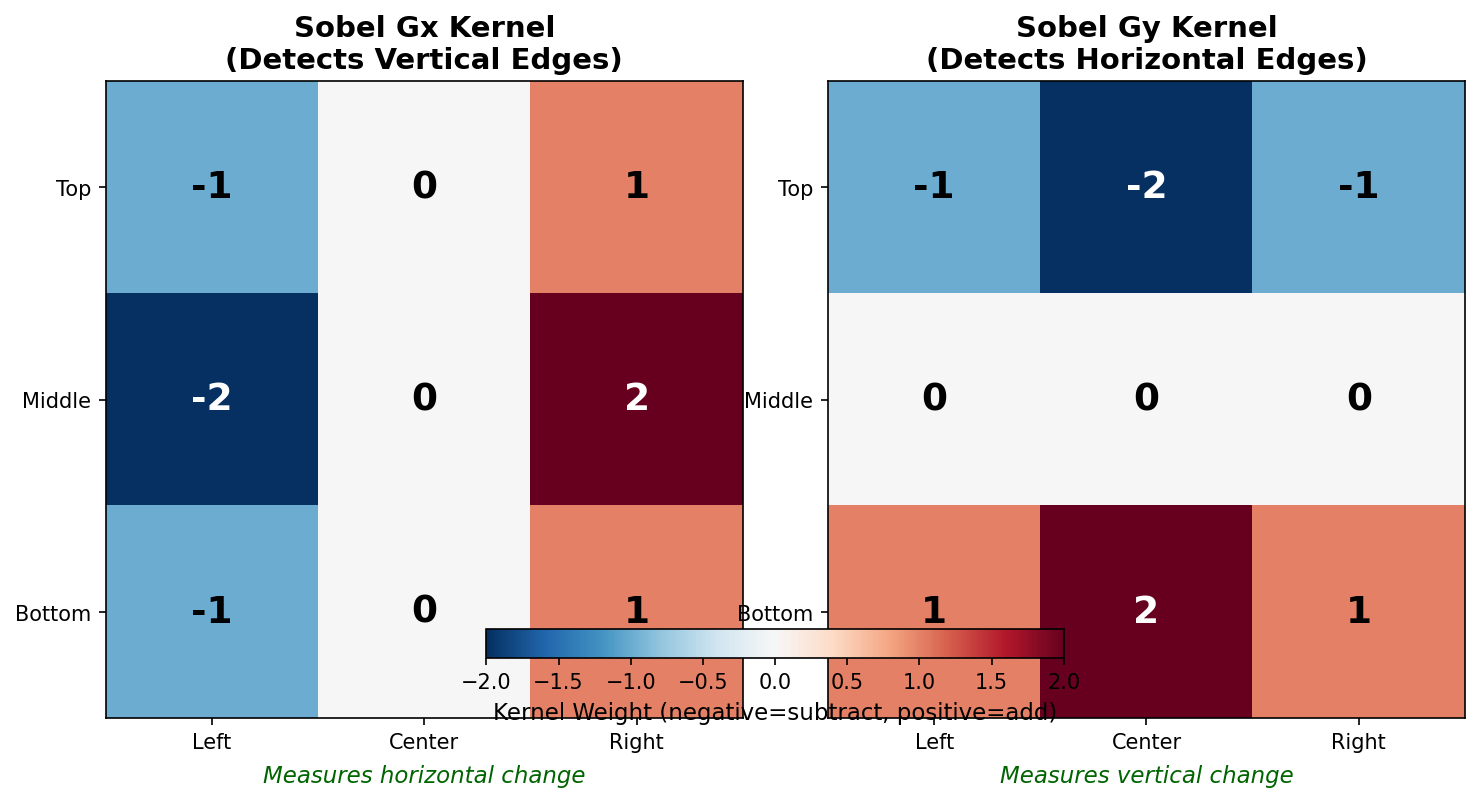
The Sobel kernels visualized with color coding. Negative values (blue) are subtracted from positive values (red). Gx measures horizontal change to detect vertical edges; Gy measures vertical change to detect horizontal edges.

Important

The naming can be confusing: Gx detects vertical edges because it measures change in the x-direction (horizontal). Similarly, Gy detects horizontal edges because it measures change in the y-direction (vertical).

Concept 3: Computing Edge Magnitude

After computing both gradients, we combine them to get the total edge strength at each pixel. The gradient magnitude uses the Euclidean distance formula:

magnitude = sqrt(Gx² + Gy²)

This ensures that edges in any direction are detected equally.

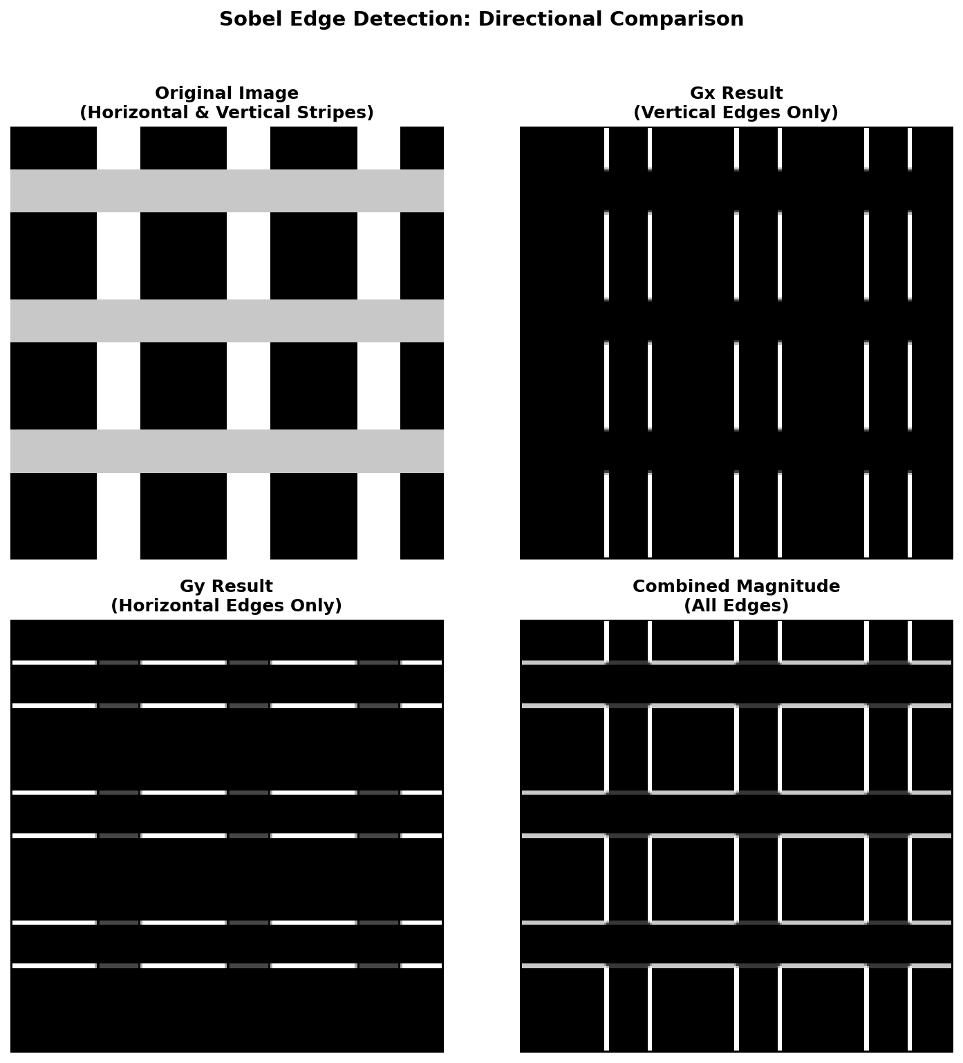
Comparing gradient directions: The original image has both horizontal and vertical stripes. Gx only shows vertical stripe edges, Gy only shows horizontal stripe edges, but the combined magnitude captures all edges.

The convolution operation works by sliding the kernel over every pixel in the image. At each position, we multiply the kernel values with the corresponding pixel values and sum them up [NumPyDocs].

Concept 4: Comparing Edge Detection Operators

The Sobel operator is not the only edge detection method. Three classic gradient-based operators are commonly compared [MarrHildreth1980]:

Roberts Cross (1965) [Roberts1965]:

Uses small 2x2 kernels. Very fast but sensitive to noise because it only considers diagonal neighbors.

Prewitt (1970) [Prewitt1970]:

Uses 3x3 kernels like Sobel but without center weighting. All neighbors have equal importance.

Sobel (1968) [Sobel1968]:

Uses 3x3 kernels with weighted center rows/columns. The weights reduce noise sensitivity by giving more importance to pixels closer to the center.

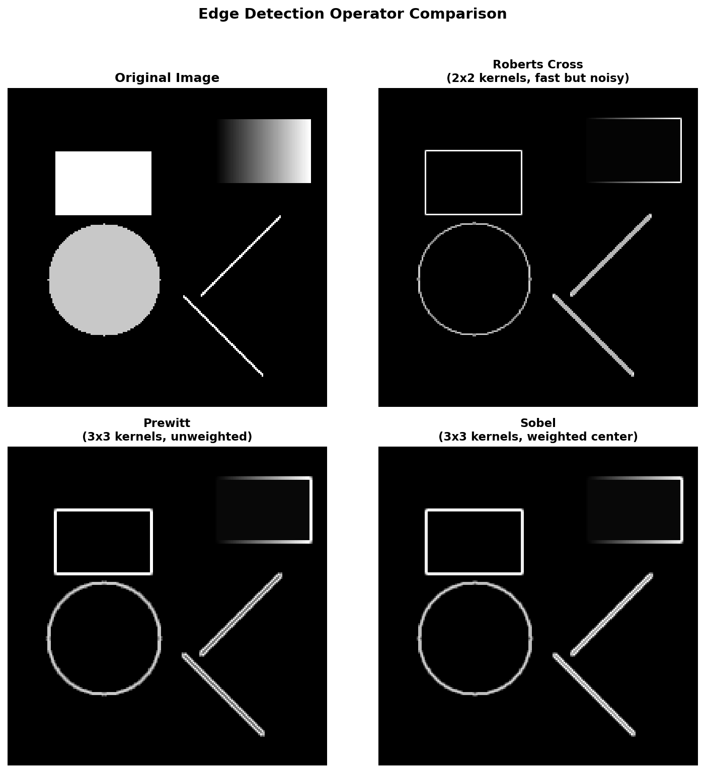
Comparing edge detection operators on the same test image. Roberts produces thinner but noisier edges. Prewitt and Sobel give similar results, with Sobel showing slightly smoother edge lines.

Did You Know?

The Canny edge detector, developed by John Canny in 1986, is often considered the gold standard for edge detection. It uses a multi-stage algorithm that includes Gaussian smoothing, gradient computation (often using Sobel), non-maximum suppression, and hysteresis thresholding [Canny1986]. While more complex, it produces cleaner edges with fewer false positives.

Hands-On Exercises

Exercise 1: Execute and Explore

Estimated time: 3-4 minutes

Run the simple_edge_detection.py script and examine the output.

python simple_edge_detection.py

Reflection Questions:

1. Why do the edges appear as white lines while everything else is black?

2. Look at the rectangle edges. Are all four sides equally bright, or do some appear stronger than others? Why might this be?

3. The circle’s edge curves in all directions. How does the Sobel operator handle diagonal edges?

Exercise 2: Modify to Achieve Goals

Estimated time: 3-4 minutes

Modify the edge detection code to achieve these goals:

Goal 1: Detect only vertical edges (ignore horizontal edges)

Goal 2: Detect only horizontal edges (ignore vertical edges)

Goal 3: Show only strong edges by applying a threshold

Exercise 3: Create from Scratch

Estimated time: 5-6 minutes

Now implement Sobel edge detection from scratch. Create your own test image with a custom pattern and apply the full edge detection pipeline.

Requirements:

1. Generate a procedural test image (any pattern you like)

2. Define the Sobel Gx and Gy kernels correctly

3. Apply convolution using nested loops

4. Compute the gradient magnitude

5. Save the result

Use the starter code in edge_detection_starter.py:

Starter code for Exercise 3

import numpy as np
from PIL import Image

# Step 1: Create your test image
height, width = 256, 256
image = np.zeros((height, width), dtype=np.float64)
# TODO: Draw your pattern here

# Step 2: Define Sobel kernels
sobel_gx = np.array([
    # TODO: Fill in the 3x3 Gx kernel
])
sobel_gy = np.array([
    # TODO: Fill in the 3x3 Gy kernel
])

# Step 3: Apply convolution
edge_magnitude = np.zeros((height, width), dtype=np.float64)
for y in range(1, height - 1):
    for x in range(1, width - 1):
        # TODO: Extract neighborhood, compute gradients, compute magnitude
        pass

# Step 4: Normalize and save
edge_normalized = (255 * edge_magnitude / edge_magnitude.max()).astype(np.uint8)
Image.fromarray(edge_normalized, mode='L').save('my_edge_detection.png')

Challenge Extension:

Implement the Prewitt operator instead of Sobel and compare the results. The Prewitt kernels use equal weights instead of the 1-2-1 pattern:

prewitt_gx = np.array([[-1, 0, 1],
                       [-1, 0, 1],
                       [-1, 0, 1]])
prewitt_gy = np.array([[-1, -1, -1],
                       [ 0,  0,  0],
                       [ 1,  1,  1]])

Summary

In this exercise, you have learned the fundamentals of edge detection:

Key Takeaways:

• Edges are locations where pixel intensity changes rapidly

• The Sobel operator uses two 3x3 kernels (Gx and Gy) to compute gradients

• Gx detects vertical edges; Gy detects horizontal edges

• Gradient magnitude sqrt(Gx² + Gy²) combines both directions

• Convolution slides the kernel over each pixel, computing weighted sums

Common Pitfalls to Avoid:

• Confusing Gx and Gy: Remember that Gx measures horizontal change to find vertical edges

• Forgetting to normalize: Raw gradient values can be very large (over 1000)

• Ignoring boundaries: The 3x3 kernel cannot be centered on edge pixels

• Using wrong data types: Use float64 for intermediate calculations to avoid overflow

References

[Sobel1968] (1,2)

Sobel, I. (1968). An isotropic 3x3 image gradient operator. Presentation at Stanford Artificial Intelligence Project.

[GonzalezWoods2018]

Gonzalez, R. C., & Woods, R. E. (2018). Digital Image Processing (4th ed.). Pearson. ISBN: 978-0-13-335672-4

[Roberts1965]

Roberts, L. G. (1965). Machine perception of three-dimensional solids. In Optical and Electro-Optical Information Processing (pp. 159-197). MIT Press.

[Prewitt1970]

Prewitt, J. M. S. (1970). Object enhancement and extraction. In B. Lipkin & A. Rosenfeld (Eds.), Picture Processing and Psychopictorics (pp. 75-149). Academic Press.

[MarrHildreth1980]

Marr, D., & Hildreth, E. (1980). Theory of edge detection. Proceedings of the Royal Society of London B, 207(1167), 187-217. https://doi.org/10.1098/rspb.1980.0020

[Canny1986]

Canny, J. (1986). A computational approach to edge detection. IEEE Transactions on Pattern Analysis and Machine Intelligence, PAMI-8(6), 679-698. https://doi.org/10.1109/TPAMI.1986.4767851

[NumPyDocs]

NumPy Developers. (2024). Array manipulation routines. NumPy Documentation. Retrieved December 7, 2025, from https://numpy.org/doc/stable/reference/routines.array-manipulation.html

[PillowDocs]

Clark, A., et al. (2024). Pillow: Python Imaging Library (Version 10.x). Python Software Foundation. https://python-pillow.org/