2.1.1 - Drawing Lines#

Duration:: 20 minutes
Level:: Beginner

Overview#

Lines are the basic building blocks of computer graphics. Drawing a line between two points seems simple, but how do we represent a continuous line using discrete pixels? In this exercise, you will learn to draw lines with NumPy and use them to create generative art patterns.

Learning Objectives

By completing this exercise, you will:

Understand line drawing algorithms and their historical context (Bresenham, DDA)
Implement parametric line interpolation using NumPy’s linspace
Create generative line art patterns through iteration
Recognize lines as fundamental primitives in computational geometry

Quick Start: Draw Your First Line#

Let’s start by drawing a single diagonal line across a canvas. This demonstrates the core concept: a line is simply a series of connected pixels.

simple_line.py - Draw a diagonal line#

import numpy as np
from PIL import Image

# Create blank canvas (grayscale image)
canvas = np.zeros((400, 400), dtype=np.uint8)

# Define line endpoints
x_start, y_start = 50, 50
x_end, y_end = 350, 350

# Calculate number of points needed
# At least one point per pixel in the longer dimension
num_points = max(abs(x_end - x_start), abs(y_end - y_start)) + 1

# Generate interpolated coordinates using linspace
# linspace creates evenly spaced points between start and end
x_coords = np.linspace(x_start, x_end, num_points).round().astype(int)
y_coords = np.linspace(y_start, y_end, num_points).round().astype(int)

# Draw line by setting pixels to white (255)
# Remember: array indexing is [row, column] which is [y, x]
canvas[y_coords, x_coords] = 255

# Save result
Image.fromarray(canvas).save('simple_line.png')

A white diagonal line on black background — A simple diagonal line from (50, 50) to (350, 350). Notice how the continuous mathematical line is represented as discrete white pixels on a black canvas.#

Tip

The key insight: Lines are interpolated points. We calculate enough points to fill every pixel along the line’s path, ensuring no gaps appear.

Core Concept 1: Line Drawing Algorithms#

The Challenge of Discrete Lines#

In mathematics, a line is defined by the equation \(y = mx + b\) or parametrically as \((x(t), y(t))\). These are continuous functions that exist at every point along the infinite real number line. But computer screens are discrete grids of pixels with integer coordinates.

How do we convert a continuous line into discrete pixels? This is the fundamental challenge of rasterization: converting vector graphics (mathematical descriptions) into raster graphics (pixel grids).

Historical Approaches

The earliest computers faced this challenge when creating vector displays and pen plotters. Two famous algorithms emerged:

DDA (Digital Differential Analyzer): Incremental algorithm that steps through one coordinate and calculates the other. Simple but requires floating-point arithmetic.
Bresenham’s Line Algorithm: Integer-only algorithm invented in 1962 by Jack Bresenham for IBM plotters. Uses only addition, subtraction, and bit shifts crucial for early hardware with no floating-point units [Bresenham1965].

Did You Know?

Bresenham’s algorithm was invented for pen plotters, which were mechanical devices that physically drew on paper. The algorithm needed to be extremely efficient because it controlled physical motors [Bresenham1965].

NumPy’s Linspace as Interpolator#

In modern Python, we do not need to implement Bresenham’s algorithm from scratch (though it is instructive to do so). Instead, NumPy provides linspace, a function that creates evenly-spaced points along a line.

# Create 5 evenly-spaced points from 0 to 10
points = np.linspace(0, 10, 5)
# Result: array([0.0, 2.5, 5.0, 7.5, 10.0])

When applied to both x and y coordinates, linspace effectively implements the parametric line equation:

\[ \begin{align}\begin{aligned}x(t) = x_0 + t(x_1 - x_0)\\y(t) = y_0 + t(y_1 - y_0)\end{aligned}\end{align} \]

where \(t \in [0, 1]\) is the parameter that varies from start (0) to end (1).

Why Round and Convert to Int?

linspace returns floating-point values, but pixel indices must be integers. We use round() before astype(int) to ensure proper rounding:

x_coords = np.linspace(50, 350, 301).round().astype(int)

Without round(), astype(int) would truncate (e.g., 2.9 → 2), causing visual artifacts.

Important

Always round before converting to int when generating pixel coordinates. Truncation creates gaps; proper rounding ensures smooth lines.

Core Concept 2: Parametric Representation#

Mathematics of Interpolation#

The parametric line equation is beautiful in its simplicity. Given two points \(P_0 = (x_0, y_0)\) and \(P_1 = (x_1, y_1)\), every point on the line can be expressed as:

\[P(t) = P_0 + t(P_1 - P_0) = (1-t)P_0 + tP_1\]

where \(t \in [0, 1]\).

When \(t = 0\): We are at \(P_0\) (start)
When \(t = 0.5\): We are at the midpoint
When \(t = 1\): We are at \(P_1\) (end)

This is called linear interpolation or “lerp” for short. It is fundamental to computer graphics, animation, and numerical methods [Foley1990].

Code Implementation#

NumPy’s linspace directly implements this:

# Create 301 evenly-spaced t values from 0 to 1
t_values = np.linspace(0, 1, 301)

# Calculate x and y using parametric equations
x_coords = x_start + t_values * (x_end - x_start)
y_coords = y_start + t_values * (y_end - y_start)

In practice, linspace simplifies this:

# Equivalent to the above, but cleaner
x_coords = np.linspace(x_start, x_end, 301)
y_coords = np.linspace(y_start, y_end, 301)

How Many Points?

Too few points create gaps; too many waste memory. The optimal number is:

num_points = max(abs(x_end - x_start), abs(y_end - y_start)) + 1

This ensures at least one point per pixel along the longer dimension [GonzalezWoods2018].

Core Concept 3: Lines as Generative Art#

Historical Context#

While line drawing was born from engineering necessity, artists quickly recognized its creative potential. Early computer art pioneers used lines as their primary expressive tool:

Vera Molnár (1960s-present): Used plotters to create geometric line compositions, exploring systematically varied parameters [Molnar1974].
Sol LeWitt (1960s-2000s): Created “wall drawings” based on simple line-drawing instructions executed by others. This conceptual approach parallels algorithmic art [LeWitt1967].
Naum Gabo (1920s-1970s): Though working with physical materials, created sculptural “constructions” using strings and lines that anticipate computational line art.

The connection is profound: algorithms are instructions, just as LeWitt’s wall drawings were instructions. The computer becomes the artist’s assistant, executing simple rules to create complex results.

From Utility to Aesthetics#

Let’s see how iteration transforms a single line into a pattern:

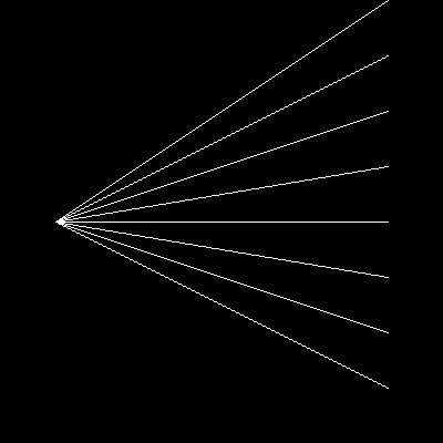
Radial pattern of lines emanating from a single point — A radial line pattern created by drawing lines from a fixed point (50, 200) to evenly-spaced points on the opposite edge. Simple iteration creates visual complexity.#

The code behind this pattern:

fixed_x, fixed_y = 50, 200
target_x = 350

for target_y in range(0, 400, 50):
    draw_line(canvas, fixed_x, fixed_y, target_x, target_y)

Key Insight: Iteration + variation = emergent pattern. We are not drawing the pattern directly; we are defining rules that generate it.

Hands-On Exercises#

Exercise 1: Execute and Explore#

Run simple_line.py and observe the output. This introduces you to the basic line drawing function.

Reflection Questions:

Why do we need round() before converting to int?
What happens if you swap the start and end points?
Why use max() when calculating num_points?

Exercise 2: Modify Parameters#

Modify simple_line.py to achieve these goals:

Goals:

Draw a horizontal line from (50, 200) to (350, 200)
Draw a vertical line from (200, 50) to (200, 350)
Draw 5 parallel diagonal lines spaced 40 pixels apart

Exercise 3: Create a Sunburst Pattern#

Create a “sunburst” pattern: lines radiating from the center to evenly-spaced points on the canvas edge.

Goal: Create a radial pattern with at least 16 lines emanating from the center (200, 200) to points on a circle.

Requirements:

Canvas size: 400×400 pixels
Center point: (200, 200)
At least 16 evenly-spaced rays
Use trigonometry to calculate endpoints

Hints:

Use np.linspace to create evenly-spaced angles from 0 to \(2\pi\)
Convert polar coordinates to Cartesian: \(x = r \cos(\theta), y = r \sin(\theta)\)
Loop through angles, drawing a line from center to each calculated endpoint
Remember to round and convert to integers

Exercise 3 starter code#

import numpy as np
from PIL import Image

def draw_line(canvas, x_start, y_start, x_end, y_end):
    # (Copy the draw_line function from previous examples)
    pass

canvas = np.zeros((400, 400), dtype=np.uint8)
center_x, center_y = 200, 200
radius = 180  # Distance from center to edge

# Your code here: create sunburst pattern
# Step 1: Create array of angles
# Step 2: Loop through angles
# Step 3: Calculate endpoint using cos/sin
# Step 4: Draw line from center to endpoint

Image.fromarray(canvas).save('sunburst.png')

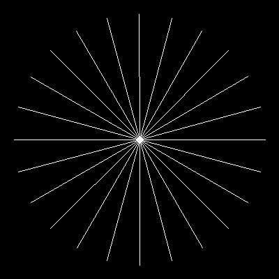
Radial sunburst pattern with 24 evenly-spaced rays — Example output: A sunburst pattern with 24 rays radiating from the center. This demonstrates how trigonometry and iteration create symmetrical generative art.#

Summary#

In this exercise, you have learned the fundamentals of line drawing in computer graphics.

Key Takeaways:

Lines are interpolated points between start and end coordinates
NumPy’s linspace provides parametric interpolation: \(P(t) = (1-t)P_0 + tP_1\)
Always round() before converting to int to avoid visual artifacts
Calculating max(abs(x_end - x_start), abs(y_end - y_start)) + 1 points ensures smooth lines
Iteration + simple rules = complex patterns (foundational principle of generative art)

Common Pitfalls to Avoid:

Forgetting to round: astype(int) truncates, not rounds. Use .round().astype(int) to avoid gaps.
Confusing (x, y) vs (row, col): Array indexing is array[row, col] which is array[y, x]. Be careful with coordinate order!
Not enough points: Using too few interpolated points creates gaps. Always calculate based on the line’s length.
Using the wrong data type: Images require dtype=np.uint8 for 0-255 pixel values.

This foundational knowledge prepares you for more complex geometric primitives. Lines combine to form triangles, polygons, and curves. The parametric thinking you have learned here extends to Bézier curves, splines, and transformations.

References#

[Bresenham1965] (1,2)

Bresenham, J. E. (1965). Algorithm for computer control of a digital plotter. IBM Systems Journal, 4(1), 25-30. https://doi.org/10.1147/sj.41.0025 [Original paper describing the famous integer-only line algorithm for pen plotters]

[NumPyLinspace]

NumPy Developers. (2024). numpy.linspace. NumPy Documentation. Retrieved January 30, 2025, from https://numpy.org/doc/stable/reference/generated/numpy.linspace.html [Official documentation for NumPy’s linear interpolation function]

[Molnar1974]

Molnár, V. (1974). Toward aesthetic guidelines for paintings with the aid of a computer. Leonardo, 7(3), 185-189. https://doi.org/10.2307/1572906 [Pioneer of computer-generated geometric art discussing systematic exploration of visual parameters]

[LeWitt1967]

LeWitt, S. (1967). Paragraphs on conceptual art. Artforum, 5(10), 79-83. [Foundational text on conceptual art where instructions/algorithms are the artwork]

[Foley1990]

Foley, J. D., van Dam, A., Feiner, S. K., & Hughes, J. F. (1990). Computer Graphics: Principles and Practice (2nd ed.). Addison-Wesley. ISBN: 978-0201121100 [Chapter 3: Output Primitives - comprehensive coverage of line drawing algorithms]

[GonzalezWoods2018]

Gonzalez, R. C., & Woods, R. E. (2018). Digital Image Processing (4th ed.). Pearson. ISBN: 978-0133356724 [Standard textbook covering image representation, interpolation, and geometric transformations]