4.1.3 Mandelbrot Set#

Duration:: 25-30 minutes
Level:: Intermediate

Overview#

The Mandelbrot set is perhaps the most famous fractal in mathematics, revealing infinite complexity from an elegantly simple formula: \(z_{n+1} = z_n^2 + c\). Named after mathematician Benoit Mandelbrot, who first visualized it using computers in 1980, this fractal has become an icon of both mathematical beauty and computational art [Mandelbrot1982]. Its discovery helped launch the popular understanding of chaos theory and fractal geometry [Gleick1987].

In this exercise, you will implement the escape-time algorithm to generate stunning Mandelbrot visualizations. You will learn how complex numbers behave under iteration and discover why some points remain bounded forever (belonging to the set) while others spiral off to infinity. This forms the foundation for understanding many other fractal systems, including Julia sets and Newton fractals.

Learning Objectives#

By the end of this exercise, you will be able to:

Understand complex number arithmetic and visualize numbers on the complex plane
Implement the Mandelbrot iteration algorithm using vectorized NumPy operations
Apply color mapping techniques to transform iteration counts into striking visualizations
Explore self-similarity by zooming into different regions of the fractal

Quick Start: See It In Action#

Run this code to generate your first Mandelbrot set visualization:

Generate the Mandelbrot set#

import numpy as np
from PIL import Image

# Create a grid of complex numbers
x = np.linspace(-2.5, 1.0, 512)
y = np.linspace(-1.5, 1.5, 512)
real, imag = np.meshgrid(x, y)
c = real + 1j * imag

# Iterate z = z^2 + c
z = np.zeros_like(c)
iterations = np.zeros(c.shape, dtype=np.int32)
for i in range(100):
    mask = np.abs(z) <= 2
    z[mask] = z[mask]**2 + c[mask]
    iterations[mask] += 1

# Map to colors and save
colors = (iterations / 100 * 255).astype(np.uint8)
Image.fromarray(colors).save('mandelbrot_basic.png')

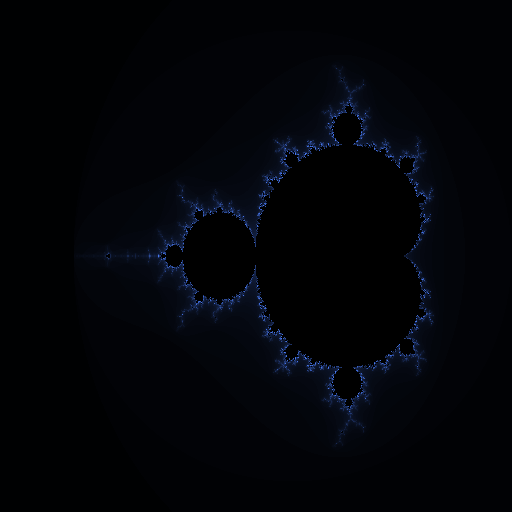
The Mandelbrot set showing the characteristic cardioid and circular bulbs in blue gradient — The Mandelbrot set rendered with a blue color gradient. The black region is the set itself, where points never escape. The colored regions show how quickly points escape, with darker colors indicating more iterations before escape.#

The iconic shape emerges: a cardioid-shaped main body connected to circular bulbs, with intricate detail at every boundary. Each pixel represents one complex number, colored according to how many iterations it took to determine whether that point belongs to the Mandelbrot set.

Core Concepts#

Concept 1: Complex Numbers and the Complex Plane#

A complex number has the form \(c = a + bi\), where \(a\) is the real part, \(b\) is the imaginary part, and \(i = \sqrt{-1}\) is the imaginary unit [Devaney1989]. We can visualize complex numbers as points on a 2D plane, where the horizontal axis represents the real part and the vertical axis represents the imaginary part.

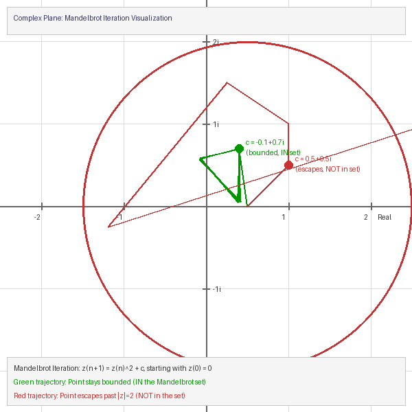
Diagram showing the complex plane with real and imaginary axes, escape boundary circle, and example iteration trajectories — The complex plane showing the escape boundary (`|z| = 2` circle) and two example trajectories. The green path stays bounded (point is IN the set), while the red path escapes (point is NOT in the set).#

In NumPy, we can create arrays of complex numbers easily:

Creating a grid of complex numbers with NumPy#

import numpy as np

# Create 1D arrays for real and imaginary values
real_values = np.linspace(-2.5, 1.0, 512)   # Real axis: -2.5 to 1.0
imag_values = np.linspace(-1.5, 1.5, 512)   # Imaginary axis: -1.5 to 1.5

# Create 2D grids
real_grid, imag_grid = np.meshgrid(real_values, imag_values)

# Combine into complex numbers: c = real + imaginary * i
c = real_grid + 1j * imag_grid  # 1j is Python's imaginary unit

print(f"Shape: {c.shape}")         # (512, 512)
print(f"Top-left corner: {c[0,0]}") # (-2.5-1.5j)

Important

Each pixel in our image corresponds to one complex number. The entire image is a “window” into the complex plane. By changing the ranges in np.linspace(), you can zoom into different regions of the plane.

Concept 2: The Mandelbrot Iteration Algorithm#

The Mandelbrot set is defined by a deceptively simple iteration formula [Mandelbrot1982]:

\[z_{n+1} = z_n^2 + c\]

Starting with \(z_0 = 0\), we repeatedly apply this formula. For each complex number \(c\), we ask: does the sequence \(z_0, z_1, z_2, ...\) stay bounded, or does it escape to infinity?

If the sequence stays bounded (|z| never exceeds 2), then \(c\) belongs to the Mandelbrot set
If the sequence escapes (|z| > 2 at some iteration), then \(c\) is outside the set

Note

Mathematically, once |z| > 2, the sequence is guaranteed to escape to infinity. This is why we use 2 as our escape threshold.

Here is the core algorithm with detailed annotations:

The Mandelbrot iteration algorithm explained#

# For a single point c, track the iteration
c = complex(-0.5, 0.5)  # Example point
z = 0                    # Always start at z_0 = 0
max_iterations = 100

for n in range(max_iterations):
    z = z**2 + c         # Apply the formula

    # Check escape condition
    if abs(z) > 2:       # |z| > 2 means this point escapes
        print(f"Point escaped after {n} iterations")
        break
else:
    # Loop completed without break - point never escaped
    print("Point is IN the Mandelbrot set")

The algorithm’s power comes from tracking the iteration count when a point escapes. Points that escape quickly get low counts, while points near the boundary take many iterations to escape. This creates the beautiful gradient patterns we see in Mandelbrot visualizations.

Did You Know?

The boundary of the Mandelbrot set has infinite length but encloses a finite area of approximately 1.5065 square units [Ewing1992]. This seemingly paradoxical property is characteristic of fractal geometry.

Concept 3: Escape Time and Color Mapping#

The escape time algorithm records how many iterations each point takes before escaping. Points inside the set never escape and receive the maximum iteration count [Peitgen1986]. This iteration count data becomes our raw material for visualization.

Different color mapping techniques produce dramatically different visual effects from the same mathematical data:

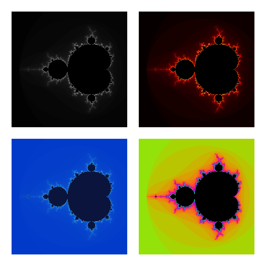
Four versions of the Mandelbrot set with different color mappings: grayscale, fire, ocean, and rainbow — The same Mandelbrot set data rendered with four different color schemes. Top-left: Grayscale. Top-right: Fire (red/orange/yellow). Bottom-left: Ocean (blue/cyan). Bottom-right: Rainbow (cyclic colors). The mathematical content is identical; only the interpretation changes.#

Applying a custom color gradient to iteration counts#

# iteration_count is our 2D array of escape times
# Normalize to 0-1 range
normalized = iteration_count / max_iterations

# Create RGB image
image = np.zeros((height, width, 3), dtype=np.uint8)

# Apply gradient: dark blue -> light blue -> white
mask_outside = iteration_count < max_iterations
image[mask_outside, 0] = (normalized[mask_outside] * 80).astype(np.uint8)   # Red
image[mask_outside, 1] = (normalized[mask_outside] * 150).astype(np.uint8)  # Green
image[mask_outside, 2] = (normalized[mask_outside] * 255).astype(np.uint8)  # Blue

# Points inside the set: black
image[~mask_outside] = [0, 0, 0]

Tip

For more visually striking results, use cyclic color mappings (like sine waves) that create bands of color. This emphasizes the fractal detail at the boundary of the set.

Hands-On Exercises#

Exercise 1: Execute and Explore#

Run the main Mandelbrot script and observe the output:

python mandelbrot_set.py

Then answer these reflection questions:

Which region of the image has the darkest colors? What does this indicate about those points?
Look at the boundary between the black region and the colored region. What do you notice about the level of detail there?
The main body of the set looks like a heart shape (cardioid). Why do you think this specific shape emerges from such a simple formula?
What do you predict would happen if you increased max_iterations from 100 to 500?

Exercise 2: Modify Parameters#

Modify the mandelbrot_set.py script to achieve these goals:

Goal 1: Zoom into the “Seahorse Valley” region centered at (-0.745, 0.113)

Goal 2: Change the color scheme from blue gradient to a “fire” colormap (red/orange/yellow)

Goal 3: Increase the resolution to 1024x1024 pixels

Exercise 3: Create a Zoom Function#

Create a reusable function that generates Mandelbrot images at any zoom level and location. Your function should:

Requirements:

Accept parameters for center point (x, y), zoom level, and image size
Calculate the appropriate viewing window from the zoom level
Return an RGB image array

Starter Code:

Starter code for zoom function#

import numpy as np
from PIL import Image

def mandelbrot_zoom(center_x, center_y, zoom_level, size=512, max_iter=200):
    """
    Generate a Mandelbrot image at the specified location and zoom.

    Parameters:
        center_x, center_y: Center point in the complex plane
        zoom_level: Magnification factor (1 = full view, 10 = 10x zoom)
        size: Image dimensions (square)
        max_iter: Maximum iterations

    Returns:
        np.ndarray: RGB image array
    """
    # TODO: Calculate x_min, x_max, y_min, y_max from center and zoom

    # TODO: Create complex grid

    # TODO: Run iteration algorithm

    # TODO: Apply color mapping

    # TODO: Return image array
    pass


# Test your function
if __name__ == '__main__':
    # Generate zoomed image
    image = mandelbrot_zoom(-0.745, 0.113, zoom_level=50)
    Image.fromarray(image).save('my_zoom.png')
    print("Zoomed image saved!")

Challenge Extension: Create Zoom Animation#

Using your zoom function, create an animated GIF that zooms into an interesting region of the Mandelbrot set.

Starter code for zoom animation#

import imageio

frames = []
target_x, target_y = -0.745, 0.113  # Seahorse valley

for i in range(60):
    zoom = 1.2 ** i  # Exponential zoom
    print(f"Generating frame {i+1}/60 at {zoom:.1f}x zoom...")
    frame = mandelbrot_zoom(target_x, target_y, zoom, size=256, max_iter=150)
    frames.append(frame)

imageio.mimsave('mandelbrot_zoom.gif', frames, fps=15)
print("Animation saved as mandelbrot_zoom.gif")

Summary#

Key Takeaways#

The Mandelbrot set is defined by the iteration \(z = z^2 + c\), where points that stay bounded belong to the set
Complex numbers can be visualized on a 2D plane, with real and imaginary axes corresponding to x and y coordinates
The escape time algorithm tracks how many iterations until |z| > 2, creating the data for visualization
Color mapping transforms iteration counts into visual representations, with many possible artistic interpretations

Common Pitfalls#

Forgetting dtype=complex128: When creating the z array, use dtype=np.complex128 to avoid precision errors
Using loops instead of vectorization: Always use NumPy masks (z[mask]) rather than Python loops for performance
Not increasing iterations when zooming: Deeper zooms reveal more detail, which requires more iterations to resolve

These common errors align with cognitive load principles [Sweller2019]: breaking down complex algorithms into smaller steps helps learners avoid overload [Mayer2020].

Next Steps#

Continue to ../../4.1.4_julia_sets/README to explore Julia sets, which use the same iteration formula but with a fixed value of c for all points. You will discover how Mandelbrot and Julia sets are mathematically connected.

References#

[Mandelbrot1982] (1,2)

Mandelbrot, B. B. (1982). The Fractal Geometry of Nature. W.H. Freeman and Company. ISBN: 978-0-7167-1186-5

[Peitgen1986]

Peitgen, H.-O., & Richter, P. H. (1986). The Beauty of Fractals: Images of Complex Dynamical Systems. Springer-Verlag. https://doi.org/10.1007/978-3-642-61717-1

[Devaney1989]

Devaney, R. L. (1989). An Introduction to Chaotic Dynamical Systems (2nd ed.). Addison-Wesley. ISBN: 978-0-8133-4085-2

[Gleick1987]

Gleick, J. (1987). Chaos: Making a New Science. Viking Press. ISBN: 978-0-14-009250-9

[Ewing1992]

Ewing, J. H., & Schober, G. (1992). The area of the Mandelbrot set. Numerische Mathematik, 61(1), 59-72. https://doi.org/10.1007/BF01385497

[Harris2020]

Harris, C. R., et al. (2020). Array programming with NumPy. Nature, 585, 357-362. https://doi.org/10.1038/s41586-020-2649-2

[Mayer2020]

Mayer, R. E. (2020). Multimedia Learning (3rd ed.). Cambridge University Press. https://doi.org/10.1017/9781316941355

[Sweller2019]

Sweller, J., van Merriënboer, J. J. G., & Paas, F. (2019). Cognitive architecture and instructional design: 20 years later. Educational Psychology Review, 31, 261-292. https://doi.org/10.1007/s10648-019-09465-5