
5.1.1 Sand Simulation#
- Duration:
18-22 minutes
- Level:
Intermediate
- Prerequisites:
Module 1.1.1 (Arrays and Images)
Overview#
Have you ever watched sand blow across a desert, each grain moving independently yet creating a mesmerizing collective pattern? In this exercise, you will build a particle system that simulates this exact phenomenon. By the end, you will understand how simple physics rules applied to thousands of independent agents can create complex, natural-looking motion.
Particle systems are one of the most versatile tools in generative art and visual effects. First developed for the “Genesis sequence” in Star Trek II: The Wrath of Khan, they now power everything from fire and smoke in video games to flocking birds in nature documentaries [Reeves1983].
Learning Objectives
By completing this exercise, you will:
Understand particle systems as collections of independent agents with state
Implement physics-based motion using position, velocity, and acceleration
Use randomness (Gaussian distribution) to create natural timing variations
Generate frame-by-frame animations and export them as animated GIFs
Quick Start: Watch the Sand Blow Away#
Let’s start by running the simulation and seeing the result. Save this code as sand_simulation.py and run it:
import random
import numpy as np
from PIL import Image
import imageio.v2 as imageio

# Create 500 particles at the center
particles = []
for _ in range(500):
    particles.append({
        'x': 150 + random.randint(0, 100),
        'y': 100 + random.randint(0, 100),
        'vx': random.uniform(-1, 2),
        'vy': random.uniform(-0.5, 0.5),
        'delay': random.randint(0, 60)
    })

frames = []
for frame in range(80):
    img = np.zeros((200, 300, 3), dtype=np.uint8)
    for p in particles:
        if p['delay'] > 0:
            p['delay'] -= 1
            color = (50, 40, 30)  # Waiting: dark
        else:
            p['x'] += p['vx']
            p['y'] += p['vy']
            p['vx'] *= 1.05  # Accelerate
            color = (194, 178, 128)  # Moving: sand color
        x, y = int(p['x']), int(p['y'])
        if 0 <= x < 297 and 0 <= y < 197:
            img[y:y+3, x:x+3] = color
    frames.append(img)

imageio.mimsave('quick_sand.gif', frames, fps=24)
After running this code, open quick_sand.gif to see the animation.
Full sand simulation with 6,700 grains accelerating rightward#
Tip
Notice how the grains start dark and motionless, then turn beige and accelerate as they begin moving. This creates the illusion of sand being swept away by wind.
Core Concepts#
What Are Particle Systems?#
A particle system is a technique for simulating fuzzy phenomena by managing large collections of small, independent objects called particles. Each particle has its own state (position, velocity, color) and follows simple rules that govern its behavior.
The key components of any particle system are:
Particles: Individual agents with properties like position, velocity, and lifetime
Emitter: The source that creates new particles (in our case, a rectangular region)
Update Rules: Physics equations that modify each particle every frame
Renderer: Code that draws each particle to the canvas
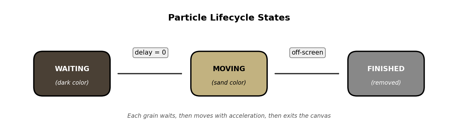
Particle lifecycle states. Diagram generated with Claude Code.#
In our sand simulation, each grain progresses through three states:
WAITING: The grain is stationary, colored dark, counting down its delay timer
MOVING: The grain is active, colored beige, accelerating to the right
FINISHED: The grain has exited the canvas and is removed from rendering
Did You Know?
William Reeves invented particle systems in 1982 at Lucasfilm to create the fiery “Genesis Effect” in Star Trek II. His paper described particles as having position, velocity, color, and age, all concepts we use today [Reeves1983].
Physics of Motion#
Our particles move according to simple physics: position changes by velocity, and velocity changes by acceleration. This is called Euler integration, one of the simplest methods for simulating motion.
The core physics equations are:
position_new = position + velocity
velocity_new = velocity × acceleration
In code, this translates to:
 1def update(self):
 2    # Update position using velocity
 3    self.x += self.velocity_x
 4    self.y += self.velocity_y
 5
 6    # Accelerate rightward (wind effect)
 7    if self.velocity_x < 1.0:
 8        self.velocity_x += 0.2  # Redirect leftward motion
 9    else:
10        self.velocity_x *= self.acceleration  # Speed up exponentially
Line 6-10 show the key physics: particles start with random velocities (some moving left, some right), but the acceleration gradually redirects them all rightward. Once moving right, they accelerate exponentially, creating the “blown away” effect.
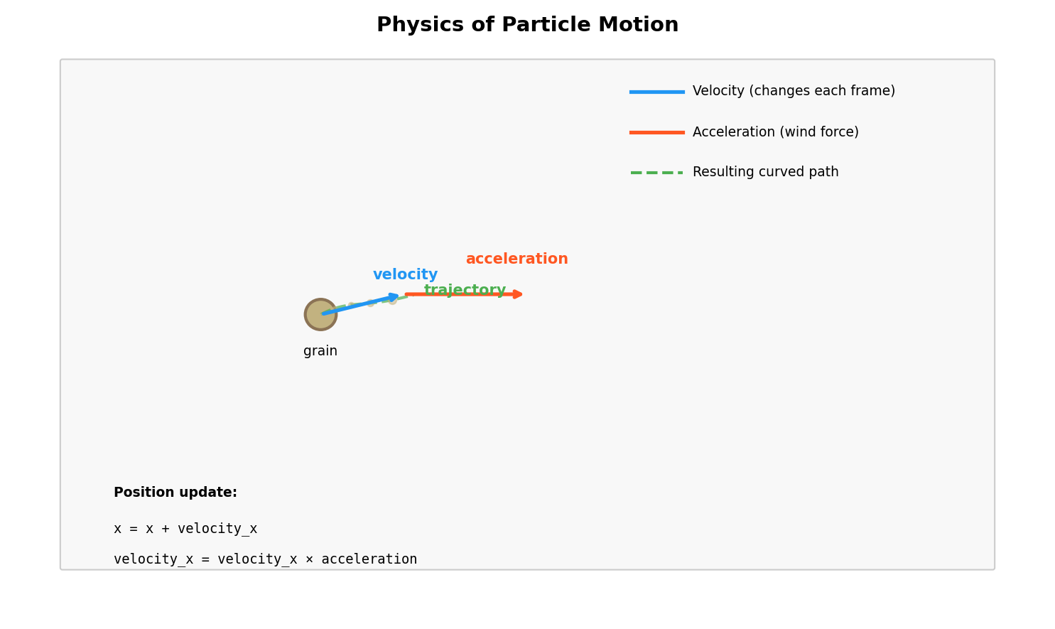
Velocity and acceleration vectors determine particle trajectory. Diagram generated with Claude Code.#
Important
We use float values for position and velocity, then convert to int only when drawing. This allows smooth sub-pixel movement that looks natural.
Creating Natural Variation with Randomness#
Real sand does not move in perfect unison. To create natural-looking motion, we introduce randomness at several levels:
Delay Distribution: Each grain waits a random time before moving
self.delay = max(0, int(random.gauss(50, 15)))
This uses a Gaussian (normal) distribution centered at 50 frames with a standard deviation of 15. Most grains start moving around frame 50, but some start early (frame 20) and some late (frame 80).
Initial Velocity Variation: Grains start with slightly different speeds
self.velocity_x = random.uniform(-1.5, 1.5)
self.velocity_y = random.uniform(-0.3, 0.3)
Color Variation: Each grain has a slightly different shade of beige
self.color = (
    base[0] + random.randint(-30, 30),
    base[1] + random.randint(-30, 30),
    base[2] + random.randint(-20, 20)
)
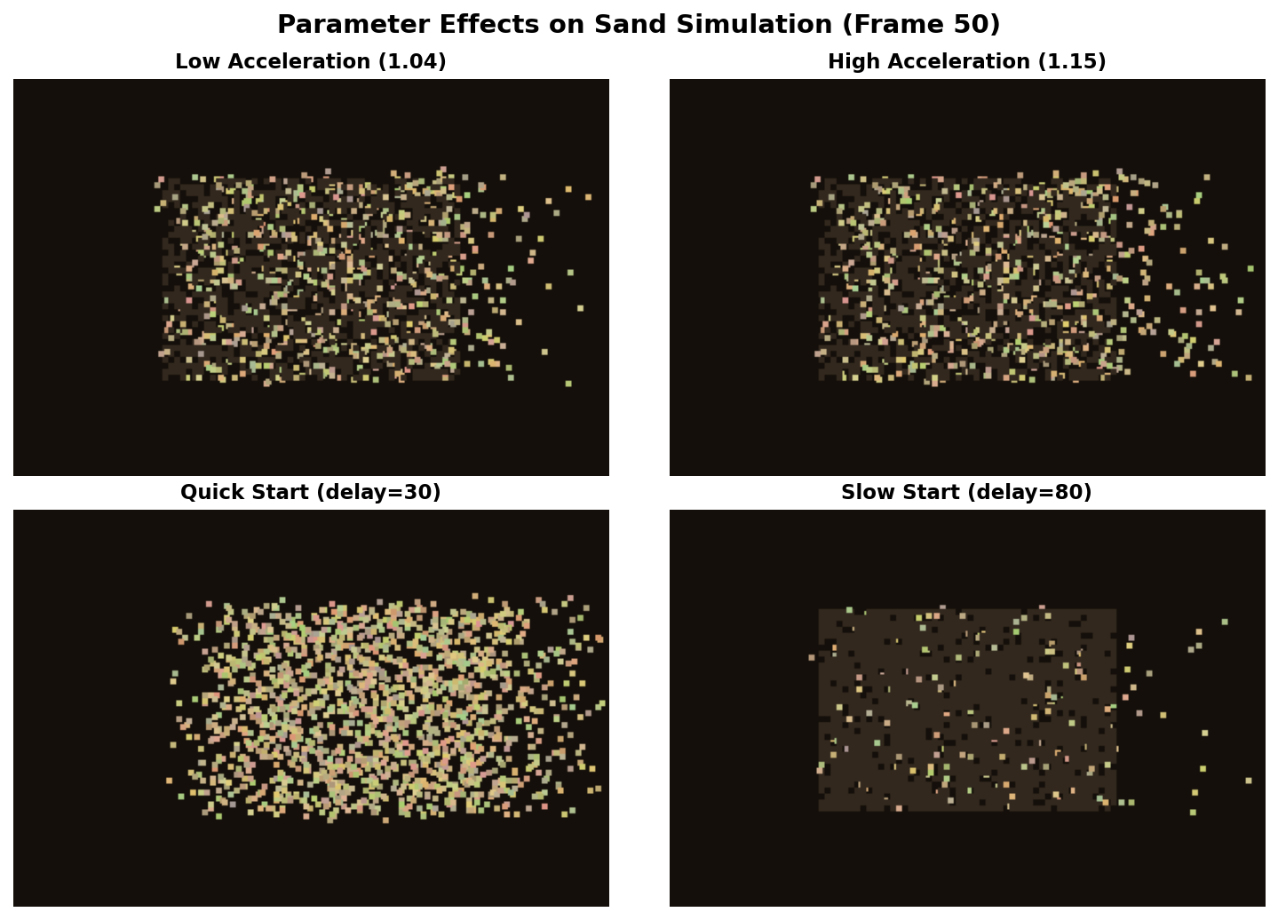
Different parameter values create distinct visual effects#
Note
The Gaussian distribution is ideal for natural phenomena because it clusters values around a mean while allowing occasional outliers, just like real-world variation.
The Complete Implementation#
Here is the full, annotated simulation code. Study how the pieces fit together:
  1"""
  2Sand Simulation: A Particle System Demonstration
  3
  4This script creates an animated sand simulation where thousands of particles
  5follow simple physics rules to create a natural wind-blown effect. Each grain
  6waits for a random time before starting to move, then accelerates rightward
  7while drifting slightly up or down.
  8"""
  9
 10import random
 11import numpy as np
 12from PIL import Image
 13import imageio.v2 as imageio
 14
 15# =============================================================================
 16# Configuration Parameters
 17# =============================================================================
 18WIDTH, HEIGHT = 600, 400          # Canvas dimensions in pixels
 19GRAIN_SIZE = 3                    # Size of each sand grain in pixels
 20NUM_FRAMES = 120                  # Total frames in the animation
 21
 22# Color definitions (RGB format)
 23BACKGROUND_COLOR = (20, 15, 10)   # Dark brown background
 24SAND_WAITING = (50, 40, 30)       # Dark color for stationary grains
 25SAND_BASE = (194, 178, 128)       # Base beige color for moving grains
 26
 27
 28# =============================================================================
 29# Sand Grain Class
 30# =============================================================================
 31class SandGrain:
 32    """
 33    Represents a single grain of sand with position, velocity, and state.
 34
 35    Each grain waits for a random delay before moving, then accelerates
 36    rightward to simulate being blown by wind.
 37    """
 38
 39    def __init__(self, x, y, target_x):
 40        # Position (using floats for smooth sub-pixel movement)
 41        self.x = float(x)
 42        self.y = float(y)
 43        self.target_x = target_x
 44
 45        # Delay before movement starts (Gaussian distribution creates natural variation)
 46        self.delay = max(0, int(random.gauss(50, 15)))
 47
 48        # Movement state
 49        self.is_moving = False
 50        self.is_finished = False
 51
 52        # Velocity components
 53        self.velocity_x = random.uniform(-1.5, 1.5)  # Initial horizontal speed
 54        self.velocity_y = random.uniform(-0.3, 0.3)  # Slight vertical drift
 55        self.acceleration = 1.08                      # Speed multiplier per frame
 56
 57        # Create slightly varied color for natural appearance
 58        self.color = (
 59            SAND_BASE[0] + random.randint(-30, 30),
 60            SAND_BASE[1] + random.randint(-30, 30),
 61            SAND_BASE[2] + random.randint(-20, 20)
 62        )
 63
 64    def update(self):
 65        """Update grain position and state for one frame."""
 66        if self.is_finished:
 67            return
 68
 69        # Count down delay before moving
 70        if self.delay > 0:
 71            self.delay -= 1
 72            return
 73
 74        # Mark as moving and update position
 75        self.is_moving = True
 76        self.x += self.velocity_x
 77        self.y += self.velocity_y
 78
 79        # Accelerate rightward (simulates wind pushing the grain)
 80        if self.velocity_x < 1.0:
 81            self.velocity_x += 0.2  # Redirect leftward motion to right
 82        else:
 83            self.velocity_x *= self.acceleration
 84
 85        # Check if grain has left the canvas
 86        if self.x >= self.target_x or self.y < 0 or self.y >= HEIGHT:
 87            self.is_finished = True
 88
 89
 90# =============================================================================
 91# Simulation Functions
 92# =============================================================================
 93def create_sand_grains(start_x, end_x, start_y, end_y):
 94    """Create a grid of sand grains covering a rectangular region."""
 95    grains = []
 96    for x in range(start_x, end_x, GRAIN_SIZE):
 97        for y in range(start_y, end_y, GRAIN_SIZE):
 98            grains.append(SandGrain(x, y, WIDTH - 2))
 99    return grains
100
101
102def draw_grains(frame, grains):
103    """Draw all grains onto the frame array."""
104    for grain in grains:
105        if grain.is_finished:
106            continue
107
108        # Choose color based on movement state
109        color = grain.color if grain.is_moving else SAND_WAITING
110
111        # Draw grain as a small square
112        x, y = int(grain.x), int(grain.y)
113        if 0 <= x < WIDTH - GRAIN_SIZE and 0 <= y < HEIGHT - GRAIN_SIZE:
114            frame[y:y + GRAIN_SIZE, x:x + GRAIN_SIZE] = color
115
116
117def run_simulation():
118    """Run the complete sand simulation and save outputs."""
119    # Create sand grains in the center of the canvas
120    grains = create_sand_grains(150, 450, 100, 300)
121    print(f"Created {len(grains)} sand grains")
122
123    frames = []
124
125    for frame_num in range(NUM_FRAMES):
126        # Create blank frame with background color
127        frame = np.full((HEIGHT, WIDTH, 3), BACKGROUND_COLOR, dtype=np.uint8)
128
129        # Update all grains
130        for grain in grains:
131            grain.update()
132
133        # Draw all grains
134        draw_grains(frame, grains)
135        frames.append(frame)
136
137        # Progress indicator
138        if frame_num % 30 == 0:
139            active = sum(1 for g in grains if not g.is_finished)
140            print(f"Frame {frame_num}/{NUM_FRAMES}, Active grains: {active}")
141
142    # Save animated GIF
143    imageio.mimsave('sand_animation.gif', frames, fps=24, loop=0)
144    print("Saved: sand_animation.gif")
145
146    # Save a snapshot from midway through the animation
147    snapshot_frame = frames[NUM_FRAMES // 3]
148    Image.fromarray(snapshot_frame).save('sand_snapshot.png')
149    print("Saved: sand_snapshot.png")
150
151
152# =============================================================================
153# Main Entry Point
154# =============================================================================
155if __name__ == '__main__':
156    run_simulation()
Key sections explained:
Lines 1-14: Configuration parameters that control the simulation
Lines 17-75: The
SandGrainclass that represents each particleLines 78-96: Helper functions to create and draw particles
Lines 99-122: The main simulation loop that generates frames
Hands-On Exercises#
Exercise 1: Execute and Observe#
Run the complete simulation and observe the output carefully.
Task
Execute sand_simulation.py and open sand_animation.gif in an image viewer. Watch the animation several times, paying attention to the details.
Reflection Questions:
Why do the grains not all start moving at the same time? What visual effect does this create?
Follow a single grain with your eyes. Does it travel in a straight line, or does it curve? What causes this?
Watch grains as they move further right. Do they speed up, slow down, or maintain constant speed?
Check the console output. How many grains does the simulation create?
Exercise 2: Modify Parameters#
Experiment with different parameter values to understand how they affect the simulation.
Task
Modify sand_simulation.py to achieve each of the following goals. Make one change at a time and observe the results.
Goals:
Make the sand blow LEFT instead of right
Make the sand FALL DOWN like gravity instead of blowing sideways
Make all grains start moving within 20 frames instead of 50
Create a “sunset” color palette with reds and oranges instead of beige
Exercise 3: Build Your Own Particle System#
Now create your own particle effect from scratch using the starter template.
Task
Using sand_simulation_starter.py as your base, implement ONE of the following particle effects:
Rain Drops: Particles spawn at the top, fall straight down with slight horizontal drift, and disappear at the bottom
Rising Bubbles: Particles spawn at the bottom, float upward with a gentle side-to-side wiggle
Confetti Burst: Particles spawn at the center, explode outward in all directions, then slow down due to friction
Requirements:
At least 100 particles
Particles should have appropriate colors for your effect
Animation should be at least 60 frames
Particles must be removed when they exit the canvas
Challenge Extension
After completing one effect, try combining multiple particle systems! For example, create fireworks by spawning a “rocket” particle that rises, then at its peak, spawns 50 confetti particles that explode outward.
Summary#
You have now built a complete particle system from scratch. This technique forms the foundation for countless visual effects, from realistic physics simulations to abstract generative art.
Key Takeaways:
Particle systems manage collections of independent agents, each with position, velocity, and state
Simple physics rules (position += velocity, velocity *= acceleration) create complex emergent behavior
Randomness using Gaussian distribution creates natural variation in timing and appearance
Animations are sequences of frames, each one updating particle positions and rendering to an array
Common Pitfalls to Avoid:
Forgetting bounds checking: Particles that go off-screen should be marked as finished, otherwise they consume memory and processing time forever
Using integers for position: Always use float for smooth motion, converting to int only when drawing pixels
Too many particles: Each particle requires computation every frame. Start with hundreds, not thousands, until you understand performance
Looking Ahead
In the next exercise, ../../../5.1.2_vortex/vortex/README, you will learn how to create circular motion and vortex effects by applying rotational forces to particles.
References#
Reeves, W. T. (1983). Particle systems: A technique for modeling a class of fuzzy objects. ACM SIGGRAPH Computer Graphics, 17(3), 359-375. https://doi.org/10.1145/964967.801167
Shiffman, D. (2012). The Nature of Code, Chapter 4: Particle Systems. https://natureofcode.com/book/chapter-4-particle-systems/
Sims, K. (1990). Particle animation and rendering using data parallel computation. ACM SIGGRAPH Computer Graphics, 24(4), 405-413.
Reynolds, C. W. (1987). Flocks, herds and schools: A distributed behavioral model. ACM SIGGRAPH Computer Graphics, 21(4), 25-34.
Pearson, M. (2011). Generative Art: A Practical Guide Using Processing. Manning Publications. ISBN: 978-1935182627
Harris, C. R., et al. (2020). Array programming with NumPy. Nature, 585, 357-362. https://doi.org/10.1038/s41586-020-2649-2
Klein, A., et al. (2024). imageio: Python library for reading and writing image data. https://imageio.readthedocs.io/
Burden, R. L., & Faires, J. D. (2015). Numerical Analysis (10th ed.). Cengage Learning. Chapter 5: Initial-Value Problems for Ordinary Differential Equations.