2.3.3 - Harmonograph Simulation

Duration:

20 minutes

Level:

Beginner-Intermediate

Overview

A harmonograph is a mechanical device that uses pendulum motion to draw beautiful, intricate patterns. Invented in the mid-19th century, these machines became popular parlor entertainment and produced drawings that were considered “automatic art.” In this exercise, you will simulate a two-pendulum harmonograph digitally, discovering how the interplay of two oscillating motions creates complex, elegant curves.

The key insight is that combining two simple periodic motions produces surprisingly complex patterns. This same principle underlies many phenomena in physics, music, and nature - from the interference patterns of waves to the orbital resonances of moons.

Learning Objectives

By the end of this exercise, you will be able to:

• Understand how two independent pendulum oscillations combine to create patterns

• Implement damped sinusoidal equations that model real pendulum physics

• Predict pattern characteristics from frequency ratios

• Create color-coded visualizations that reveal the dynamics of pendulum motion

Quick Start

Let us create a harmonograph pattern immediately:

simple_harmonograph.py

import numpy as np
from PIL import Image, ImageDraw
from pathlib import Path

SCRIPT_DIR = Path(__file__).parent
CANVAS_SIZE = 512
CENTER = CANVAS_SIZE // 2

# Pendulum X parameters
FREQ_X, AMP_X, PHASE_X = 3, 200, 0
# Pendulum Y parameters
FREQ_Y, AMP_Y, PHASE_Y = 2, 200, np.pi / 2

DAMPING = 0.002
t = np.linspace(0, 100, 5000)
decay = np.exp(-DAMPING * t)

# Calculate damped oscillations
x = CENTER + AMP_X * np.sin(FREQ_X * t + PHASE_X) * decay
y = CENTER + AMP_Y * np.sin(FREQ_Y * t + PHASE_Y) * decay

image = Image.new('RGB', (CANVAS_SIZE, CANVAS_SIZE), (10, 10, 20))
draw = ImageDraw.Draw(image)
points = list(zip(x.astype(int), y.astype(int)))
draw.line(points, fill=(100, 200, 255), width=1)
image.save(SCRIPT_DIR / 'simple_harmonograph.png')

Download simple_harmonograph.py and run it to generate:

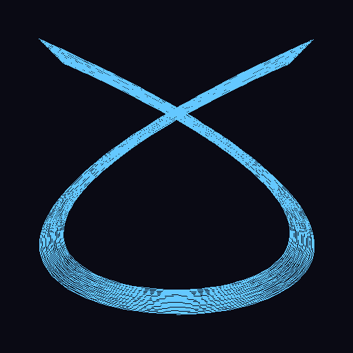
A harmonograph with 3:2 frequency ratio. The pattern shows how the two pendulums interact - one swinging faster than the other - while both gradually lose energy to damping.

Tip

The frequency ratio (3:2 in this example) determines the fundamental character of the pattern. Try different ratios to discover the variety of patterns a harmonograph can create!

Core Concepts

Concept 1: Two Pendulums, One Pattern

A harmonograph uses two pendulums swinging at right angles to each other. One pendulum controls the horizontal (x) position, the other controls the vertical (y) position. The pen traces out a curve as both pendulums swing simultaneously.

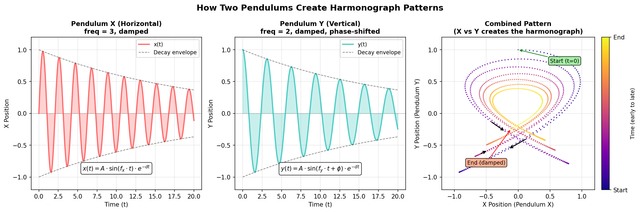
The harmonograph principle: Two independent oscillations (X and Y) combine to create a complex pattern. The damping causes both oscillations to decay over time, which is why the pattern spirals inward. Diagram generated with Claude - Opus 4.5.

The Mathematical Model

Each pendulum’s motion is described by a damped sinusoid:

\[ \begin{align}\begin{aligned}x(t) = A_x \cdot \sin(f_x \cdot t + \phi_x) \cdot e^{-d \cdot t}\\y(t) = A_y \cdot \sin(f_y \cdot t + \phi_y) \cdot e^{-d \cdot t}\end{aligned}\end{align} \]

Where:

• A is amplitude (how far the pendulum swings)

• f is frequency (how fast the pendulum swings)

• phi is phase (where in its swing the pendulum starts)

• d is damping (how quickly the swing decays due to friction)

• t is time

Implementing the equations in NumPy

import numpy as np

# Time array
t = np.linspace(0, 100, 5000)

# Damping factor (exponential decay)
damping = 0.002
decay = np.exp(-damping * t)

# X and Y positions (damped oscillations)
x = amplitude_x * np.sin(freq_x * t + phase_x) * decay
y = amplitude_y * np.sin(freq_y * t + phase_y) * decay

Did You Know?

The harmonograph was invented by Scottish mathematician Hugh Blackburn around 1844. By the 1890s, harmonographs were popular drawing toys. Some elaborate versions used three or four pendulums to create even more complex patterns [Ashton2003].

Concept 2: Frequency Ratios and Pattern Character

The ratio between the X and Y frequencies is the most important parameter. Simple ratios like 1:1, 2:1, or 3:2 produce closed, recognizable patterns. More complex ratios create intricate designs that take longer to repeat.

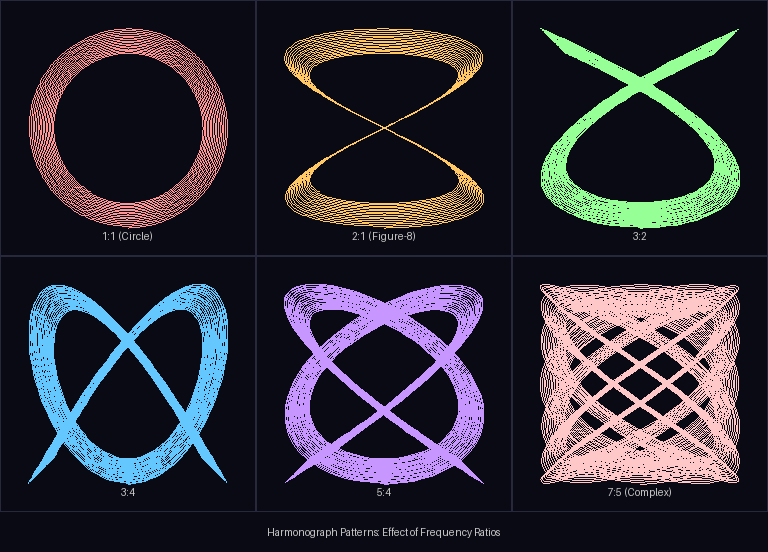
Effect of frequency ratios on harmonograph patterns. Simple ratios (1:1, 2:1) create simple shapes; complex ratios (5:4, 7:5) create more intricate patterns. Diagram generated with Claude - Opus 4.5.

Common Frequency Ratios

Ratio	Pattern Type	Musical Analogy
1:1	Circle or ellipse	Unison
2:1	Figure-8	Octave
3:2	Three-lobed pattern	Perfect fifth
4:3	Four-lobed pattern	Perfect fourth
5:4	Five-lobed pattern	Major third

Important

The frequency ratios used in harmonographs correspond exactly to the frequency ratios that define musical intervals! A 3:2 ratio sounds like a perfect fifth on a piano. This connection between visual patterns and musical harmony was recognized by early harmonograph enthusiasts [Ashton2003].

Concept 3: Damping and Energy Decay

Real pendulums lose energy over time due to friction and air resistance. This damping causes the amplitude to decrease exponentially, making the pattern spiral inward toward the center. The damping factor controls how quickly this happens.

The exponential decay function

import numpy as np

damping = 0.002  # Small value = slow decay
t = np.linspace(0, 100, 5000)

# Decay factor starts at 1.0 and decreases toward 0
decay = np.exp(-damping * t)

# At t=0: decay = 1.0 (full amplitude)
# At t=50: decay ≈ 0.90 (90% amplitude)
# At t=100: decay ≈ 0.82 (82% amplitude)

Effects of different damping values:

• Low damping (0.001): Slow decay, many loops before pattern fades

• Medium damping (0.005): Balanced decay, clear spiral inward

• High damping (0.01): Fast decay, pattern quickly converges to center

Note

Without damping, a harmonograph would trace the same path forever. The damping creates the characteristic “fading” effect that makes each drawing unique - like a signature of the pendulum’s energy dissipation.

Hands-On Exercises

Exercise 1: Execute and Explore

Run the simple_harmonograph.py script and observe the output.

python simple_harmonograph.py

Reflection Questions

1. What frequency ratio is used? How does it relate to the pattern shape?

2. Where does the pattern start (at t=0) and where does it end?

3. What role does the phase difference (PHASE_Y = pi/2) play?

Answers

1. 3:2 ratio: The X pendulum completes 3 full cycles for every 2 cycles of the Y pendulum. This creates a pattern with interlocking loops characteristic of this ratio.

2. Start and end: The pattern starts at the outer edge (when decay = 1.0) and spirals inward toward the center as the decay factor approaches 0. At the end, both oscillations have nearly zero amplitude.

3. Phase difference: The pi/2 (90-degree) phase shift means the Y pendulum starts at its maximum position when X is at zero. Without this phase shift, the pattern would collapse to a diagonal line. Phase shifts create the “openness” of the pattern.

Exercise 2: Modify Parameters

Using simple_harmonograph.py as a starting point, achieve these goals:

Goal 1: Create a figure-8 pattern (what frequency ratio?)

Goal 2: Create a more complex pattern with 5 lobes

Goal 3: Make the pattern decay faster (reach center sooner)

Hint for Goal 1

A figure-8 is created by a 2:1 frequency ratio. Change FREQ_X = 2 and FREQ_Y = 1.

Hint for Goal 2

Try a 5:4 ratio (FREQ_X = 5, FREQ_Y = 4) or a 5:3 ratio for different 5-lobed patterns.

Hint for Goal 3

Increase the DAMPING value. Try DAMPING = 0.01 for fast decay, or 0.005 for moderate.

Complete Solutions

# Goal 1: Figure-8 pattern
FREQ_X = 2
FREQ_Y = 1

# Goal 2: Five-lobed pattern
FREQ_X = 5
FREQ_Y = 4

# Goal 3: Faster decay
DAMPING = 0.01  # Increased from 0.002

Exercise 3: Create a Color-Fading Harmonograph

Create a harmonograph where the color fades from bright to dark as the pendulum loses energy. This visualizes the energy dissipation!

Requirements

• Start with a bright color (cyan, magenta, or your choice)

• Fade to a darker shade as time progresses

• Use the decay factor to drive the color change

Starter Code

import numpy as np
from PIL import Image, ImageDraw
from pathlib import Path

SCRIPT_DIR = Path(__file__).parent
CANVAS_SIZE = 512
CENTER = CANVAS_SIZE // 2
BASE_COLOR = (100, 255, 255)  # Bright cyan

# Generate oscillations with decay
t = np.linspace(0, 100, 5000)
decay = np.exp(-0.003 * t)
x = CENTER + 200 * np.sin(5 * t) * decay
y = CENTER + 200 * np.sin(4 * t + np.pi/2) * decay

image = Image.new('RGB', (CANVAS_SIZE, CANVAS_SIZE), (10, 10, 20))
draw = ImageDraw.Draw(image)

for i in range(1, len(t)):
    # TODO: Calculate faded color based on decay[i]
    color = BASE_COLOR  # Replace with fading calculation

    draw.line([(int(x[i-1]), int(y[i-1])), (int(x[i]), int(y[i]))],
             fill=color, width=1)

image.save(SCRIPT_DIR / 'my_colored_harmonograph.png')

Hint 1: Simple Color Fading

Multiply each color component by the decay value:

color = tuple(int(c * decay[i]) for c in BASE_COLOR)

Hint 2: Color Interpolation

For a smoother transition between two colors:

START_COLOR = (100, 255, 255)  # Cyan
END_COLOR = (20, 40, 80)       # Dark blue

def get_faded_color(decay_value):
    r = int(START_COLOR[0] * decay_value + END_COLOR[0] * (1 - decay_value))
    g = int(START_COLOR[1] * decay_value + END_COLOR[1] * (1 - decay_value))
    b = int(START_COLOR[2] * decay_value + END_COLOR[2] * (1 - decay_value))
    return (r, g, b)

Complete Solution

import numpy as np
from PIL import Image, ImageDraw
from pathlib import Path

SCRIPT_DIR = Path(__file__).parent
CANVAS_SIZE = 512
CENTER = CANVAS_SIZE // 2

# Color gradient: bright -> dark
START_COLOR = (100, 255, 255)
END_COLOR = (20, 40, 80)

def get_faded_color(decay_value):
    """Interpolate between START and END colors based on decay."""
    r = int(START_COLOR[0] * decay_value + END_COLOR[0] * (1 - decay_value))
    g = int(START_COLOR[1] * decay_value + END_COLOR[1] * (1 - decay_value))
    b = int(START_COLOR[2] * decay_value + END_COLOR[2] * (1 - decay_value))
    return (r, g, b)

t = np.linspace(0, 100, 5000)
decay = np.exp(-0.003 * t)
x = CENTER + 200 * np.sin(5 * t) * decay
y = CENTER + 200 * np.sin(4 * t + np.pi/2) * decay

image = Image.new('RGB', (CANVAS_SIZE, CANVAS_SIZE), (10, 10, 20))
draw = ImageDraw.Draw(image)

for i in range(1, len(t)):
    color = get_faded_color(decay[i])
    draw.line([(int(x[i-1]), int(y[i-1])), (int(x[i]), int(y[i]))],
             fill=color, width=1)

image.save(SCRIPT_DIR / 'colored_harmonograph_solution.png')

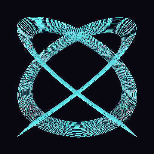
The color-fading harmonograph shows energy dissipation visually. Bright cyan (high energy) fades to dark blue (low energy) as the pendulum decays.

Challenge Extension

A. Animated Harmonograph: Create a GIF showing the harmonograph being drawn over time, as if watching a real pendulum at work.

B. Three-Pendulum Harmonograph: Add a third pendulum that modulates the x or y position, creating even more complex patterns.

C. Musical Harmonograph: Create a series of patterns using frequency ratios that correspond to musical intervals (octave, fifth, fourth, third).

D. Interactive Explorer: Build a script that accepts command-line arguments for frequency ratios and damping, allowing quick exploration of parameter space.

Summary

Key Takeaways

• A harmonograph combines two damped sinusoidal oscillations to create complex patterns

• The frequency ratio (fx:fy) determines the basic character of the pattern

• Damping causes the pattern to spiral inward as energy dissipates

• Phase difference prevents the pattern from collapsing to a line

• These concepts connect to physics (pendulums, waves), music (harmonic ratios), and art (generative patterns)

Common Pitfalls

• Zero phase difference: If both pendulums start at the same phase, the pattern degenerates to a line. Always include a phase offset.

• Too much damping: High damping values cause the pattern to collapse too quickly. Start with small values (0.001-0.005).

• Equal frequencies: A 1:1 ratio with the same phase produces a circle or ellipse - interesting but simple.

• Not enough points: Too few points (NUM_POINTS) creates a jagged curve. Use 3000+ for smooth results.

References

[Ashton2003] (1,2)

Ashton, A. (2003). Harmonograph: A Visual Guide to the Mathematics of Music (2nd ed.). Walker & Company. ISBN: 978-0802714091 [Comprehensive guide to harmonograph history, construction, and mathematical principles]

[Cundy1961]

Cundy, H. M., & Rollett, A. P. (1961). Mathematical Models (2nd ed.). Oxford University Press. [Classic reference on mathematical curves including harmonograph patterns]

[Weisstein_Lissajous]

Weisstein, E. W. (2024). Lissajous Curve. MathWorld - A Wolfram Web Resource. Retrieved November 30, 2025, from https://mathworld.wolfram.com/LissajousCurve.html [Mathematical foundation for parametric curves]

[NumPyLinspace]

NumPy Developers. (2024). numpy.linspace documentation. NumPy v1.26 Manual. Retrieved November 30, 2025, from https://numpy.org/doc/stable/reference/generated/numpy.linspace.html [Official documentation for generating evenly spaced arrays]

[NumPyExp]

NumPy Developers. (2024). numpy.exp documentation. NumPy v1.26 Manual. Retrieved November 30, 2025, from https://numpy.org/doc/stable/reference/generated/numpy.exp.html [Exponential function for damping calculations]

[PillowDocs]

Clark, A., et al. (2024). Pillow: Python Imaging Library (Version 10.2.0) [Computer software]. Python Software Foundation. https://python-pillow.org/ [Image processing library used for drawing]

[Pearson2011]

Pearson, M. (2011). Generative Art: A Practical Guide Using Processing. Manning Publications. ISBN: 978-1-935182-62-5 [Modern generative art techniques including parametric curves]

[Klemens2010]

Klemens, B. (2010). The Harmonograph. Make Magazine, 23, 124-127. [Practical guide to building physical harmonographs]