2.1.3 - Drawing Circles

Duration:

20 minutes

Level:

Beginner

Overview

This exercise teaches you how to draw circles using distance calculations instead of plotting individual pixels. You will learn the mathematical definition of a circle: all points at a fixed distance from a center. By measuring how far each pixel is from a center point, we can decide which pixels belong inside the circle and color them.

Learning Objectives:

1. Understand how the Euclidean distance formula defines circles mathematically

2. Use np.ogrid to create efficient coordinate grids for vectorized calculations

3. Apply boolean masking to select and color pixels inside a shape

4. Extend the technique to create composite patterns with multiple circles

Quick Start

Let’s jump straight in and create a circle. Run this script to see the result:

circle.py - Drawing a circle with distance calculations

import numpy as np
from PIL import Image

# Configuration
CANVAS_SIZE = 512
CENTER_X, CENTER_Y = 256, 256
RADIUS = 150
CIRCLE_COLOR = [255, 128, 0]  # Orange

# Step 1: Create coordinate grids
Y, X = np.ogrid[0:CANVAS_SIZE, 0:CANVAS_SIZE]

# Step 2: Calculate squared distance from center
square_distance = (X - CENTER_X) ** 2 + (Y - CENTER_Y) ** 2

# Step 3: Create mask for pixels inside the circle
inside_circle = square_distance < RADIUS ** 2

# Step 4: Create canvas and apply color
canvas = np.zeros((CANVAS_SIZE, CANVAS_SIZE, 3), dtype=np.uint8)
canvas[inside_circle] = CIRCLE_COLOR

# Step 5: Save
Image.fromarray(canvas, mode='RGB').save('circle.png')

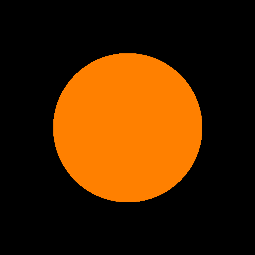
Output: A 150-pixel radius orange circle centered on a 512x512 canvas.

Tip

What you just did: You used the Pythagorean theorem to determine which pixels lie within 150 pixels of the center point (256, 256). Every pixel where distance < radius gets colored orange. This vectorized approach processes all 262,144 pixels simultaneously, making it far more efficient than a nested loop checking each pixel individually.

Core Concepts

Concept 1: The Distance Formula

A circle is mathematically defined as all points at a fixed distance (the radius) from a center point. For any pixel at position (x, y) and a circle centered at (cx, cy), we calculate the Euclidean distance:

\[d = \sqrt{(x - cx)^2 + (y - cy)^2}\]

A pixel is inside the circle if d < radius.

Important

Optimization Trick: Computing square roots is computationally expensive. Since we only need to compare distances (not measure them), we can compare squared values instead:

(x - cx)² + (y - cy)² < radius²

This is mathematically equivalent but avoids the costly sqrt() operation for every pixel. Early computer graphics used this optimization extensively due to limited hardware [Bresenham1977].

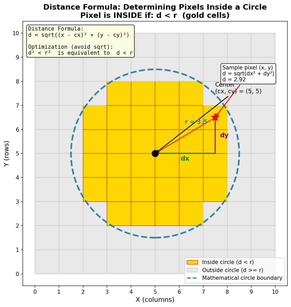
Visualizing the distance formula: Gold pixels are inside the circle (d < r), gray pixels are outside (d >= r). The dx and dy components combine via the Pythagorean theorem to give the total distance d. Diagram generated with Claude Code.

Concept 2: Coordinate Grids with np.ogrid

To calculate distances for all pixels efficiently, we need arrays containing the X and Y coordinates of every pixel. NumPy’s np.ogrid creates these “open grids” in a memory-efficient way [NumPyDocs2024]:

Y, X = np.ogrid[0:512, 0:512]

This creates two arrays:

• Y is a column vector of shape (512, 1) containing values 0 to 511

• X is a row vector of shape (1, 512) containing values 0 to 511

When used in arithmetic operations, NumPy’s broadcasting automatically expands these to full 512x512 arrays, computing the result for every pixel coordinate combination.

Note

Alternative approaches:

• np.meshgrid creates full 2D arrays (uses more memory)

• np.indices creates a 3D array of shape (2, height, width)

For most circle rendering, np.ogrid is the most memory-efficient choice.

Concept 3: Boolean Masking for Shape Selection

The comparison square_distance < RADIUS ** 2 produces a boolean array of the same shape as the canvas:

inside_circle = square_distance < RADIUS ** 2
# Result: 2D array of True/False values

This “mask” acts like a stencil. When we write:

canvas[inside_circle] = CIRCLE_COLOR

NumPy assigns CIRCLE_COLOR only to pixels where inside_circle is True. This is called boolean indexing or fancy indexing and is a powerful pattern for selective array modification [Harris2020].

Did You Know?

Boolean masking is the foundation for many image processing operations. Photo editing tools like “magic wand” selection use similar distance-based masks to select regions of similar color. In machine learning, masks are used to focus attention on specific parts of an image [Gonzalez2018].

Hands-On Exercises

Exercise 1: Execute and Explore

Run circle.py and observe the output. Then answer these reflection questions:

Reflection Questions:

1. What happens if you change RADIUS from 150 to 50? To 250?

2. Why do we compare square_distance < RADIUS ** 2 instead of calculating the actual distance with sqrt()?

3. How would you move the circle to the bottom-right corner of the canvas?

Exercise 2: Modify to Achieve Goals

Starting with the Quick Start code, complete these modification tasks:

Task A: Create a small circle in the top-left quadrant

• Radius: 50 pixels

• Center: approximately (100, 100)

• Color: Keep orange or choose your own

Task B: Create a blue circle

• Change the color to blue (hint: blue is the third channel in RGB)

Task C: Create two circles side by side

• Red circle on the left (center around x=150)

• Green circle on the right (center around x=360)

• Both with radius 100

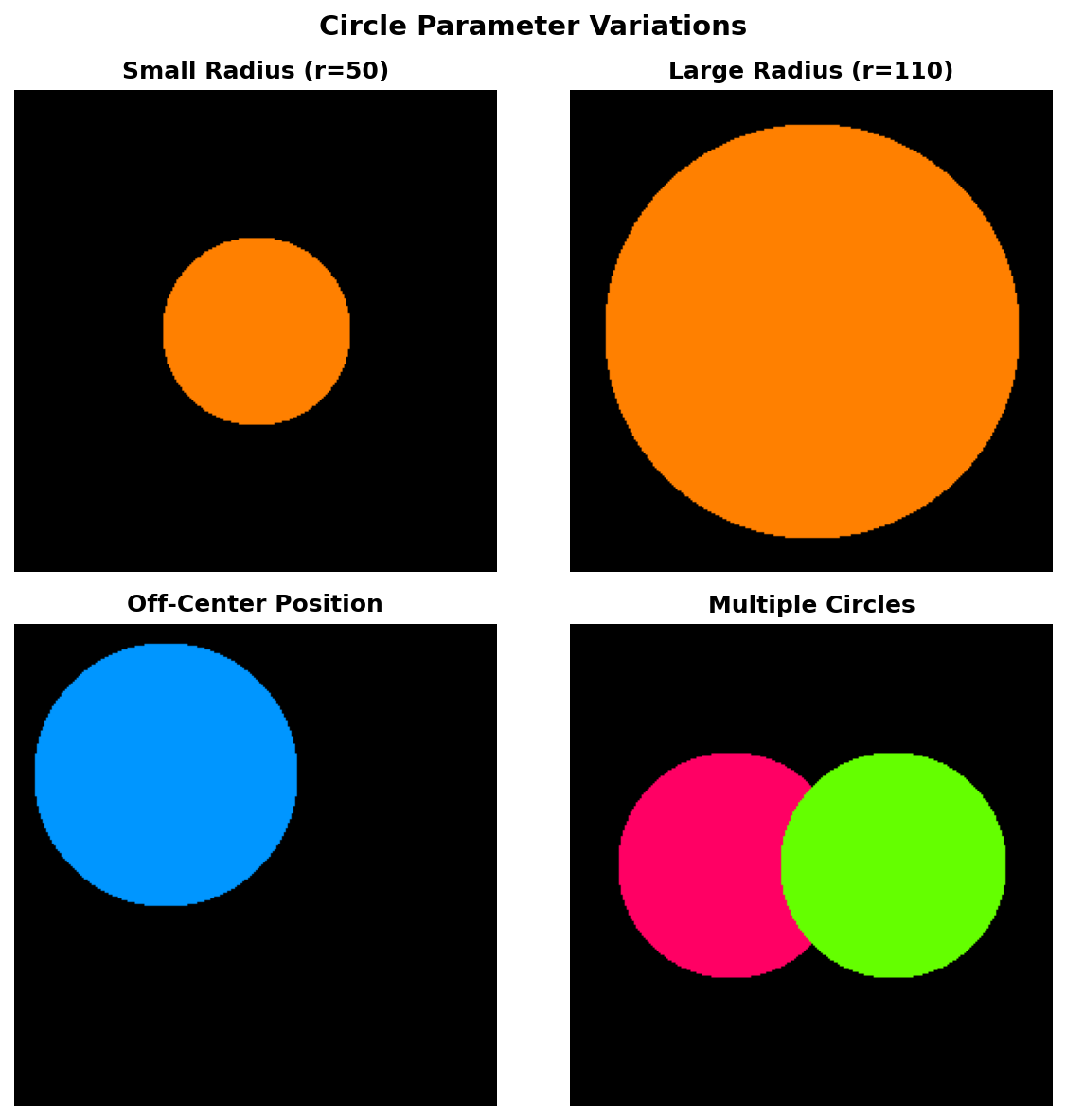
Examples of circle parameter variations: different radii, positions, and multiple circles on a single canvas.

Exercise 3: Create from Scratch - Concentric Circles

Create a bulls-eye pattern with 5 concentric circles using alternating red and white colors.

Requirements:

• Canvas size: 512x512 pixels

• Center: (256, 256)

• 5 circles with radii: 200, 160, 120, 80, 40 pixels

• Alternating colors: red, white, red, white, red (outermost to innermost)

Starter code:

concentric_circles_starter.py

import numpy as np
from PIL import Image

CANVAS_SIZE = 512
CENTER_X, CENTER_Y = 256, 256

# Define radii (largest to smallest)
RADII = [200, 160, 120, 80, 40]

# Define colors (alternating red and white)
RED = [255, 0, 0]
WHITE = [255, 255, 255]
COLORS = [RED, WHITE, RED, WHITE, RED]

# Create coordinate grids
Y, X = np.ogrid[0:CANVAS_SIZE, 0:CANVAS_SIZE]
square_distance = (X - CENTER_X) ** 2 + (Y - CENTER_Y) ** 2

canvas = np.zeros((CANVAS_SIZE, CANVAS_SIZE, 3), dtype=np.uint8)

# TODO: Loop through RADII and COLORS to draw circles
# Hint: Draw from largest to smallest so smaller circles overlay larger ones

Image.fromarray(canvas, mode='RGB').save('concentric_circles.png')

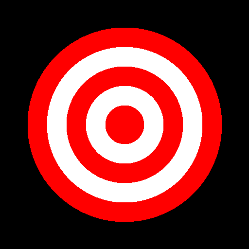
Expected output: A bulls-eye pattern with 5 concentric circles in alternating red and white colors.

Challenge Extension

Ready for a creative challenge? These patterns are inspired by techniques used in generative art [Pearson2011]. Try recreating one of these advanced patterns:

Option A: Four-Circle Flower

Create a flower-like pattern by drawing 4 overlapping circles positioned at the top, bottom, left, and right of a central point. Use a gradient color scheme (dark red to bright yellow).

Option B: Gradient Rings

Modify the concentric circles to use a smooth color gradient from the outer edge (dark) to the center (bright). Instead of just 5 colors, use a loop to create many thin rings with incrementally changing colors.

Option C: Off-Center Tunnel

Create a “tunnel” effect by drawing concentric circles where each successive circle has a slightly shifted center point, creating a perspective illusion.

Summary

Key Takeaways:

1. Circles are distance-defined: A pixel is inside a circle if its distance from the center is less than the radius.

2. Squared distance optimization: Avoid expensive sqrt() by comparing squared distances: d² < r² is equivalent to d < r.

3. np.ogrid creates efficient coordinate grids that leverage NumPy’s broadcasting for vectorized calculations.

4. Boolean masking selects pixels: Comparison operations create True/False arrays that act as stencils for selective coloring.

5. Drawing order matters: For overlapping shapes, draw from back (largest) to front (smallest) to achieve proper layering.

This exercise follows cognitive load principles by introducing concepts incrementally: first distance, then grids, then masking [Paas2020].

Common Pitfalls:

Warning

• Forgetting to square the radius: Using square_dist < RADIUS instead of square_dist < RADIUS ** 2 will create a tiny circle.

• Drawing circles in wrong order: For concentric patterns, always draw largest first; otherwise smaller circles get hidden.

• Integer overflow: For very large canvases, (X - CENTER)² + (Y - CENTER)² can overflow if using np.int32. Use np.int64 or np.float64 for safety.

References

[Harris2020]

Harris, C. R., et al. (2020). Array programming with NumPy. Nature, 585(7825), 357-362. https://doi.org/10.1038/s41586-020-2649-2 [Foundational paper on NumPy’s array operations and broadcasting]

[Gonzalez2018]

Gonzalez, R. C., & Woods, R. E. (2018). Digital Image Processing (4th ed.). Pearson. ISBN: 978-0-13-335672-4 [Standard reference for image processing algorithms including distance transforms]

[Foley1990]

Foley, J. D., van Dam, A., Feiner, S. K., & Hughes, J. F. (1990). Computer Graphics: Principles and Practice (2nd ed.). Addison-Wesley. [Classic text on computer graphics including circle rasterization algorithms]

[Bresenham1977]

Bresenham, J. E. (1977). A linear algorithm for incremental digital display of circular arcs. Communications of the ACM, 20(2), 100-106. [Historical context: Bresenham’s efficient circle algorithm for early computers]

[NumPyDocs2024]

NumPy Developers. (2024). numpy.ogrid documentation. NumPy Reference. Retrieved January 30, 2025, from https://numpy.org/doc/stable/reference/generated/numpy.ogrid.html

[Pearson2011]

Pearson, M. (2011). Generative Art: A Practical Guide Using Processing. Manning Publications. ISBN: 978-1-935182-62-5 [Practical introduction to generative art techniques including shape rendering]

[Paas2020]

Paas, F., & van Merriënboer, J. J. G. (2020). Cognitive-load theory: Methods to manage working memory load in the learning of complex tasks. Current Directions in Psychological Science, 29(4), 394-398. [Pedagogical research supporting scaffolded learning approach]